multi-class classification
multi-class classifiers, one-against-rest solutions, trained combiners
PRTools and LibSVM should be in the path
Download the m-file from here. See http://37steps.com/prtools for more.
Contents
Preparation
delfigs;       % delete existing figures
gridsize(300); % make accurate scatterplots
randreset;     % set fized seed for random generator for reporducability

% generate 2d 8-class training set
train = gendatm(250)*cmapm([1 2],'scale');
% generate test set
test  = gendatm(1000)*cmapm([1 2],'scale');
% rename PRTools qdc, include regularisation
qda   = setname(qdc([],[],1e-6),'QDA')*classc;
Multi-class classifiers
Multi-class classifiers are usually based on class models, e.g. class wise esimate probability density functions (PRTools examples are qdc, ldc, parzendc and mogc) or optimise a multi-class decision function, e.g. neural networks. The support vector classifier offered by LibSVM can also be considered as an example.
figure;
scatterd(train);    % show the training set
axis equal;
w = train*qda;      % train by QDA
e = test*w*testc;   % find classification error
plotc(w);           % show decision boundaries
title([getname(w) ' (' num2str(e,'%5.3f)')])
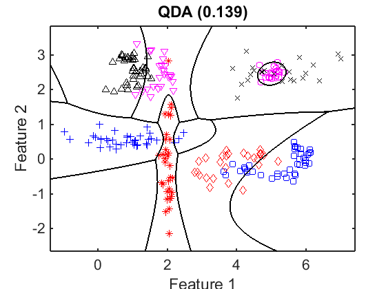
This plot shows the non-linear decision boundaries on top of the training set. They are based on the normal distributions estimated for each of the classes. Note that for some regions on the left it is not clear to which class they are assigned. The classification error estimated by the test set is shown in the title.
figure;
scatterd(train);    % show the training set
axis equal;
plotc(w,'col');     % show class domains
title([getname(w) ' (' num2str(e,'%5.3f)')])
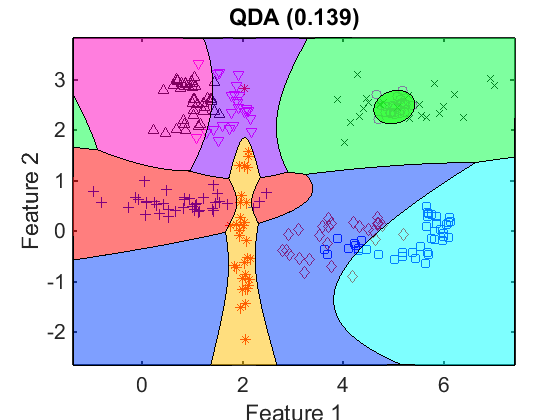
Here every class domain is indicated by a color. By an artifact of the procedure the two classes on the top right are given the same color.
figure;
scatterd(train);    % show the training set
axis equal;
w = train*libsvc;   % train by LIBSVM
e = test*w*testc;   % find classification error
plotc(w,'col');     % show class boundaries
title([getname(w) ' (' num2str(e,'%5.3f)')])
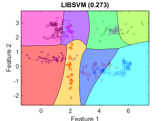
Although the basis SVM is a linear classifier, the multi-class solution for LIBSVM shows slight non-linear class borders. It suggests that in its design a non-linear kernel is used. The multi-class LIBSVM yields very often good results and is surprisingly fast in training.
One-against-rest classifiers
Many classifiers like the Fisher's Linear Discriminant and the traditional support vector machine (fisherc and svc in PRTools) offer primiarily a 2-class discriminant. In a multi-class setting they offer don't perform well, as the rest-class may dominate the result.
figure;
scatterd(train);    % show the training set
axis equal;
w = train*fisherc;  % train by FISHERC
e = test*w*testc;   % find classification error
plotc(w,'col');     % show class domains
title([getname(w) ' (' num2str(e,'%5.3f)')])
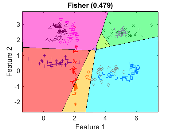
The multi-class solution found for the one-against-rest implementation of Fisher shows clearly its linear nature. The test result shown in the title is disappointing. Note that some class domains are degenerated in the centre of the plot.
figure;
scatterd(train);    % show the training set
axis equal;
w = train*(fisherc*fisherc);  % train by FISHERC*FISHERC
e = test*w*testc;   % find classification error
plotc(w,'col');     % show class domains
title([getname(w) ' (' num2str(e,'%5.3f)')])
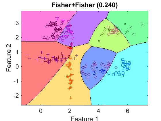
Combining the linear Fisher classifiers by, azgain, Fisher, produces a non-linear result.
figure;
scatterd(train);    % show the training set
axis equal;
w = train*svc;      % train by SVC
e = test*w*testc;   % find classification error
plotc(w,'col');     % show class domains
title([getname(w) ' (' num2str(e,'%5.3f)')])
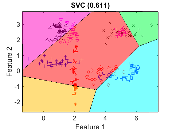
Also the multi-class version of the linear SVM shows bad results. Some class domains are not available at all.
Post-processing One-against-rest classifiers by a trained combiner
The result of a 8-class classifier is a matrix of 8 columns showing the class memberships of every object to the 8 classes. This matrix can be used as an input for an 8-dimensional multi-class classifier in a second attempt to improve the 8-class problem. Here it is shown how this may improve the disappointing results of the multi-class implementations of the Fisher and SVM classifiers shown above.
figure;
scatterd(train);          % show the training set
axis equal;
w = train*(fisherc*qda);  % train by Fisher, combine by QDA
e = test*w*testc;         % find classification error
plotc(w,'col');           % show class domains
title([getname(w) ' (' num2str(e,'%5.3f)')])
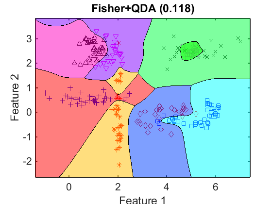
Using the quadratic postprocessing by QDA, which may also be understood as a trained combiner, the results for Fisher improve considerably: an error decrease form 0.479 to 0.118. Note that this is also better than the result of QDA alone (0.139).
figure;
scatterd(train);          % show the training set
axis equal;
w = train*(svc*qda);      % train by SVC, combine by QDA
e = test*w*testc;         % find classification error
plotc(w,'col');           % show class domains
title([getname(w) ' (' num2str(e,'%5.3f)')])
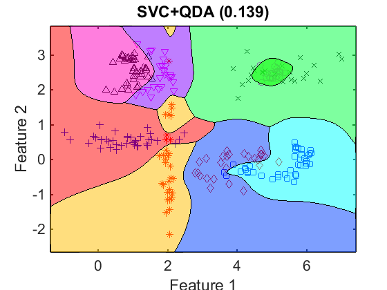
Also the linear SVC classifier improves significantly by the QDA postprocessing, but it obtains exactly the same result as for QDA alone (0.139).
figure;
scatterd(train);          % show the training set
axis equal;
w = train*(libsvc*qda);   % train by LIBSVC, combine by QDA
e = test*w*testc;         % find classification error
plotc(w,'col');           % show class domains
title([getname(w) ' (' num2str(e,'%5.3f)')])
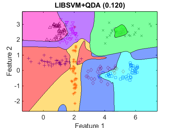
LIBSVM profits from the postprocessing as well: 0.273 to 0.120. Here we have two different multi-class classifiers for which the sequential combination is better (0.120) than each of them separately (0.139 and 0.273)
Post-processing multi-class classifiers by a trained combiner
Finally it is illustrated that applying QDA twice may cause overtraining as the postprocessing deteriorates the result.
figure;
scatterd(train);          % show the training set
axis equal;
w = train*(qda*qda);      % train by QDA, combine by QDA
e = test*w*testc;         % find classification error
plotc(w,'col');           % show class domains
title([getname(w) ' (' num2str(e,'%5.3f)')])
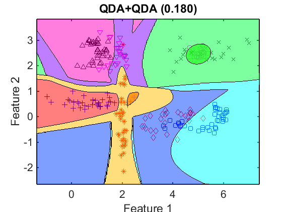
Applying QDA twice deteriorates the preformance: 0.139 to 0.180. The plot show also clear indications of ovetraining as at some places the domain of a remote class pops up.