bayes_classifier
Example of the Bayes classifier, learning curves and the Bayes error
PRTools should be in the path.
Download the m-file from here. See http://37steps.com/prtools for more.
Contents
Initialisation
delfigs
gridsize(300); % needed to show class borders accurately
randreset;     % take care of reproducability
Define dataset based on 4 normal distributions
% Covariance matrices
G = {[1 0; 0 0.25],[0.02 0; 0 3],[1 0.9; 0.9 1],[3 0; 0 3]};
% Class means
U = [1 1; 2 1; 2.5 2.5; 2 2];
% Class priors
P = [0.2 0.1 0.2 0.5];
Note that the the first three classes have small prior probabilities, and the probability of the background class is much larger.
Show maximum densities (not the sum!!) (standard Matlab)
This part of the code may be skipped. It is only needed for generating the 3D density plot.
% Domain of interest
x1 = -2:.1:6; x2 = -1.5:.1:5.5;
% Make a grid
[X1,X2] = meshgrid(x1,x2);
% Compute maximum density times prior probs for the 4 classes
F = zeros(numel(x2)*numel(x1),1);
for n=1:numel(G)
  F = max(F,P(n)*mvnpdf([X1(:) X2(:)],U(n,:),G{n}));
end
% Create plot
F = reshape(F,length(x2),length(x1));
surf(x1,x2,F);
caxis([min(F(:))-.5*range(F(:)),max(F(:))]);
axis([min(x1) max(x1) min(x2) max(x2) 0 max(F(:))])
xlabel('x1'); ylabel('x2'); zlabel('Maximum Probability Density');
title('3D view of the weighted densities.')
fontsize(14);
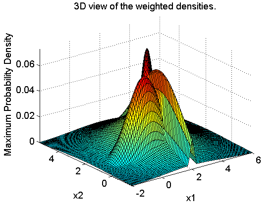
The 3D plot shows for every point of the grid the maxima of the four density functions, each multiplied by their class priors.
Compute Bayes classifier by PRTools
U = prdataset(U,[1:numel(G)]'); % create labeled dataset for class means
U = setprior(U,P);              % add class priors
G = cat(3,G{:});                % put covariance matrices in 3D array
w = nbayesc(U,G);               % Bayes classifier
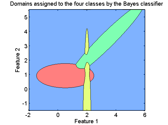
Show class domains according to Bayes classifier
figure;
axis equal
axis([min(x1) max(x1) min(x2) max(x2)]);
plotc(w,'col');
box on;
xlabel('Feature 1');
ylabel('Feature 2');
title('Domains assigned to the four classes by the Bayes classifier')
fontsize(14);
Show classifiers in prior weighted density plot
figure;
axis equal
axis([min(x1) max(x1) min(x2) max(x2)]);
plotm(w); % plot weighted density map
plotc(w); % show classifier boundaries
box on
title('Weighted density plots and the Bayes classifier')
fontsize(14);
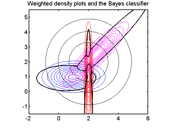
Note that the classifier passes exactly the points of equal densities of the classes.
Computation of the Bayes error
If the distributions are known the Bayes error  can be computed by integrating the areas of overlap. Here this is done be a Monte Carlo procedure: a very large dataset of a
  objects per class, is generated from the true class distributions and tested on the Bayes classifier. The standard deviation of this estimate is
n = 1000000;
a = gendatgauss(n*ones(1,4),U,G);
f = a*w*testc;
s = sqrt(f*(1-f)/n);
fprintf('The estimated Bayes error is %6.4f with standard deviation %6.4f\n',f,s);
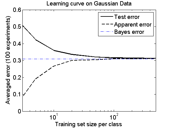
The estimated Bayes error is 0.3098 with standard deviation 0.0005
The learning curve
Here it is shown how the expected classification error approximates the Bayes error for large training set sizes. It is eeseential that a classifier is used that can model the true class distributions. In this case this is fulfilled as the true distributions are normal and the classifier, qdc, can model them.
figure;
a = gendatgauss(10000*ones(1,4),U,G); % generate 10000 objects per class
e = cleval(a,qdc,[3 5 10 20 50 100 200 500],100);
plote(e);
hold on;
feval(e.plot,[min(e.xvalues) max(e.xvalues)],[f f],'b-.');
legend off
legend('Test error','Apparent error','Bayes error')
fontsize(14);